Ingesting time series data
This is a blog post series focused on IoT
- Part I: Introduction
- Part II: Ingesting data (this post)
- Part III: Querying data
The dataset
The dataset consists of simulated messages sent from trucks. Each message looks like this:
1
2
3
4
5
6
7
8
9
10
11
12
13
14
15
16
17
18
19
{
    "latitude": 47.445301,
    "longitude": -122.296307,
    "speed": 30,
    "speed_unit": "mph",
    "temperature": 38,
    "temperature_unit": "F",
    "EventProcessedUtcTime": "2019-04-14T05:50:34.3338468Z",
    "PartitionId": 0,
    "EventEnqueuedUtcTime": "2019-04-14T05:49:38.9890000Z",
    "IoTHub": {
        "MessageId": null,
        "CorrelationId": null,
        "ConnectionDeviceId": "truck-01.659",
        "ConnectionDeviceGenerationId": "636908177760737590",
        "EnqueuedTime": "2019-04-14T05:49:38.8800000Z",
        "StreamId": null
    }
}
You can see that the messages have been enriched with some additional properties from Azure IoT Hub, but in essence, the messages are JSON objects with information about lat/lon, speed and temperature.
The dataset consits of about 114 million messages.
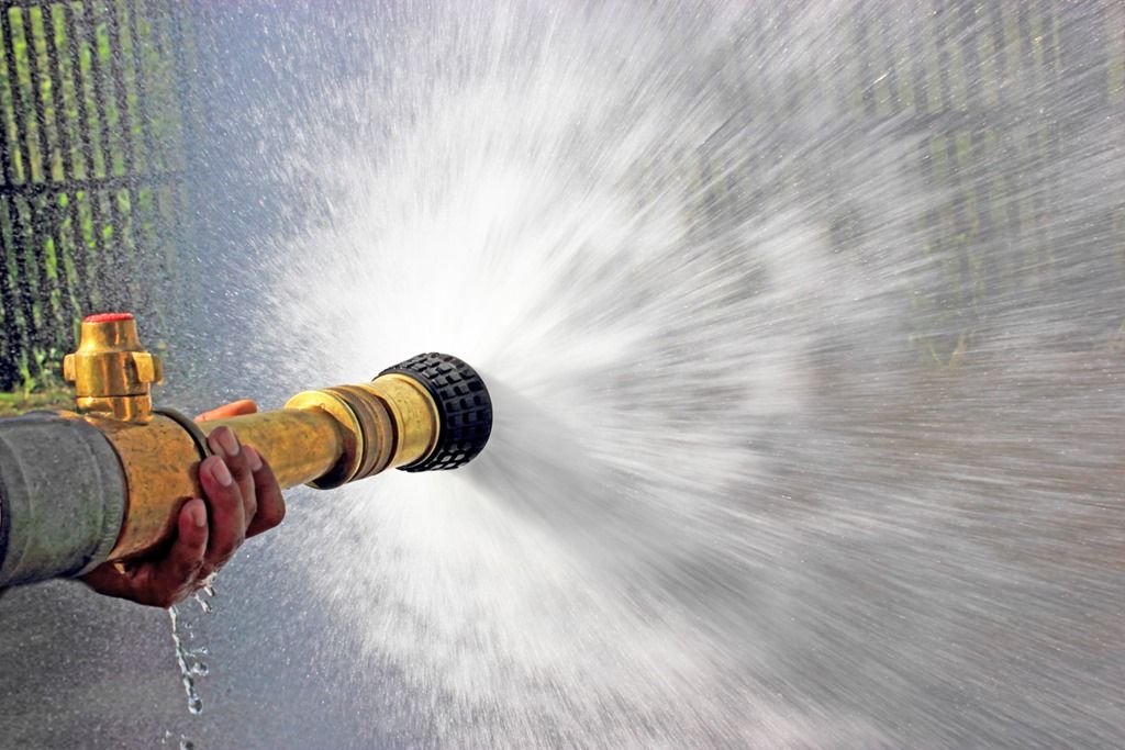
Never stick your head in front of the fire hose
As a general principle, you should never deploy your custom code in between your ingestion pipeline. This is mostly because in IoT projects, you will typically have thousands of devices sending data at the same time, which makes your ingestion pipeline look like a large firehose of messages. Inserting your custom code in the middle of the firehose requires you to engineer your code to account for large scalability, paralellization, no-message loss, and many other problems which are hard to solve.
 Don’t stick your head in front of this. Let your cloud services handle ingestion out of the box and let them handle the problem of paralellization, throughput and message processing.
Avoiding custom code in your pipeline is sometimes not possible. Sometimes you need to transform the messages, decompress/debatch them, or enrich them with data from other systems. In such cases you’ll have no option but to stick your head in front of the firehose. But for the purposes of this exercise, we will try to avoid doing that. We’ll try to implement our ingestion with as much out-of-the-box as possible.
Database setup
Azure Data Explorer
I will be running the steps in this blog post (and the next one, where I’ll deal with queries) on a shared ADX cluster. This is a cluster provided by the ADX engineering team to me for free. I don’t know how much capacity it has, all I know is that this is a cluster shared with other tenants, and I’ve been advised by the engineering team to not expect too much performance out of it. So I will be assuming the performance of this cluster will be similar to the lowest-priced ADX cluster (~300 USD/month) or worse.
Timescale
I am running Timescale on an Azure Database for PostgreSQL. It is running 4 vCores and has a total storage capacity of 106Gb. Assuming the ADX cluster is on the low-price tier (2 vCPU D11 v2 instances, which is the lowest price entrypoint at ~300 USD/month), I am scaling PostgreSQL to a similar price point of 300 bucks.
Both PostgreSQL and ADX are offered as platform-as-a-service from Microsoft and are fully managed by Microsoft. I don’t have to deal with any infrastructure problems and they can be provisioned automatically via ARM in minutes. I do not have to manage any storage, networking or VMs for any of the 2 databases.
Ingesting with Azure Data Explorer
Azure Data Explorer (ADX for short) provides several out of the box features to ingest data. For details about these ingestion methods, see HERE. All my data is exported into large blob files, so I used ADX’s blob ingest feature to bulk-import the data.
Preparing the ADX database
ADX works with tables. So the first thing I had to do was to create a table for all my Truck data:
1
.create tables Trucks (deviceId:string, timestamp:datetime, latitude:float, longitude:float, speed:float, speed_unit:string, temperature:float, temperature_unit:string)
JSON messages don’t fit tabular formats well. So the next step is to tell ADX how to map my JSON messages into the table above. ADX does this by implementing table mappings:
1
.create table Trucks ingestion json mapping 'TrucksMapping' '[{"column":"deviceId","path":"$.IoTHub.ConnectionDeviceId"}, {"column":"timestamp","path":"$.IoTHub.EnqueuedTime"}, {"column":"latitude","path":"$.latitude"}, {"column":"longitude","path":"$.longitude"}, {"column":"speed","path":"$.speed"}, {"column":"speed_unit","path":"$.speed_unit"}, {"column":"temperature","path":"$.temperature"}, {"column":"temperature_unit","path":"$.temperature_unit"}]'
Update: for production scenarios, use data type double instead of float_. This is because_ float is a 32-bit number, whereas double utilises 64 bits.
With this configuration, every time I push a JSON message from a truck, ADX will automatically flatten it into the table format I defined for the Trucks table.
To ingest the data, I used ADX’s native ingest command. This command takes a path to Azure blob storage, parses it and ingests it. Coupled with the async command, the database will immediately return an operationId, which you can use to consult the status of the import operation while it runs in the background:
1
2
3
4
5
.ingest async into table Trucks (
  h'https://luisdeltrucks.blob.core.windows.net/trucks/0_742175f33d85471281626b9816bd6f64_1.json',
    h'https://luisdeltrucks.blob.core.windows.net/trucks/0_b32e2f3120d84ecf926539c9054da9bd_1.json')
    with (jsonMappingReference = "TrucksMapping")
    with (format = "json")
Note that, by default, ADX enforces a 1 hour timeout on control commands. Ingest is a control command. This timeout is not extendable. Therefore, if your data is large and the import process takes more than 1 hour to complete, you’ll have to split your dataset into multiple files like I did above.
| Ingested rows | 114.5 million |
| Data size (sum of blob size) | 55.3 GB |
| Ingestion time | 1hour 9minutes |
Ingesting with Timescale
Since Timescale runs on top of PostgreSQL, and I vouched for platform-as-a-service in the previous post, I decided to use Timescale on Azure as a managed service. You can find the instructions to provision a Timescale db instance on Azure HERE.
Timescale also offers some features to ingest data (see HERE). Unfortunately none of these methods allow me to import JSON data from blob storage (you do have a feature to import CSV files, but since I don’t have my data in that format, I could not use it). So in the case of Timescale, I did have to write some code and stick my head in front of the firehose.
Once I provisioned my Timescale instance, I created a hypertable for Trucks data:
1
2
3
4
5
6
7
8
9
10
11
12
13
CREATE TABLE Trucks
(
    latitude numeric(9,6) NOT NULL,
    longitude numeric(9,6) NOT NULL,
    speed integer NOT NULL,
    speed_unit varchar(5) NOT NULL,
    temperature numeric(6,3) NOT NULL,
    temperature_unit varchar(2) NOT NULL,
    EventProcessedUtcTime TIMESTAMPTZ NOT NULL,
    ConnectionDeviceId varchar(200) NOT NULL
);

SELECT create_hypertable('trucks', 'eventprocessedutctime', chunk_time_interval => interval '1 hour');
Finally, I wrote this Python code to handle the bulk-import of data:
| Ingested rows | 113.7 million |
| Data size | 52.8 Gb |
| Ingestion time | 2hours 15minutes |
Note that the dataset in Timescale is slightly smaller than in ADX. This is because I imported a small data file into ADX which I did not import into Timescale. Later it was too late to correct this error and I did not want to re-run the data ingestion. However, the datasets have more or less the same sizes and this minor variation should not make a big difference.
Timescale took almost twice the time to import the dataset. This is a good illustration about why you should not stick your head in front of the firehose. I suppose Microsoft’s native blob storage import is signficantly more efficient than my Python code.
(I’m sure Microsoft has invested much more engineering time in making the blob import, compared to the time it took me to write this Python code :). So if you have a suggestion on how to improve the timescale.py script, open up a PR in GitHub or drop a comment below).
Update: Best practice for large-blob ingestion. My dataset consists of 2 large blob files: one is 47GB in size and the other is 8.1GB. Databases will have problems crunching through such large files. Specifically to ADX, the system will assign only 1 core to the ingest process per file. Therefore, issuing multiple ingest commands is much more efficient. The same problem plagues the Timescale import, as my Python script needs to parse the large files sequentially. During the import process, the Postgres instance never achieved more than 30% resource utilisation, so I estimate the system could have processed 3 files concurrently to achieve max resource utilization. As a rule of thumb, try to make your files 1 GB in size.
How do distributed databases scale?
In the previous post, I mentioned that time series databases like ADX or Timescale perform better than traditional RDBMS. What is the magic that makes this happen? There is a lot of engineering work being done behind the covers, but in essence, the reason is partitioning.
Partitioning is a concept whereby a database splits its dataset into pieces and stores the pieces as individual entities. Different compute nodes will hold one or more of these partitions. The partitioning is happening under the covers and is abstracted from the user (aka the application). The application asks for the data it needs, and the database is responsible for identifying the partitions on which the entire result set of the query lives. In essence, partitioning allows databases to benefit from paralellization techniques which boost query performance.
How does ADX distribute data?
ADX partitions data on Extents. ADX decides how to split the data into extents. In our case, the data for the Trucks table has been split into 3 extents only. This decision was made by the database itself:
1
2
.show table Trucks extents
| project ExtentId, TableName, OriginalSize, ExtentSize, CompressedSize, IndexSize
| ExtentId | TableName | OriginalSize | ExtentSize | CompressedSize | IndexSize |
|---|---|---|---|---|---|
| ba89f060-03f0-41d5-9417-fe1d2f4cf80e | Trucks | 3404972669 | 877430252 | 811758880 | 65671372 |
| 6d3ae8c4-ba81-4bd1-a5b9-6e6a20a206df | Trucks | 4129668544 | 1050480421 | 964886304 | 85594117 |
| 633b4c4d-6b58-41c4-a888-c800af5a23f3 | Trucks | 4149010294 | 1066112399 | 984692640 | 81419759 |
A word on data compression
Pay attention to ExtentId 633b4c4d-6b58-41c4-a888-c800af5a23f3. Its OriginalSize is reported as 4.1GB. However, CompressedSize is just 984MB. Index size is 81MB. Compression ratio is slightly above 4:1. This means that the database helps you save storage costs. Although storage is typically regarded as very cheap in the cloud, on large-scale IoT scenarios (where you might be ingesting terabytes of data per day) your storage costs will add up. Compression is your friend.
The other benefit of having efficient compression is that you can afford to have verbose messages without having to pay a price in terms of storage costs. Verbose messages are good. Verbosity increases the self-explanatory characteristics of messages and makes them easier to understand. It also increases the message size. With ADX, I’ve seen very verbose messages achieve a compression of 30:1, which means you can have messages with extended verbosity and still be able to store them in a cost-effective way.
How does Timescale distribute data?
Timescale also implements partitioning. The name for it is chunk. By default, chunks are based on the timestamp of the messages and they will consist of periods of 7 days. Given that my test dataset was generated within a period of 24 hours, using Timescale’s default chunking configuration would have meant that all messages would have landed in the same partition. For that reason, I specified a custom chunk time interval while creating the hypertable (see code above). Timescale created 1-hour chunks of data:
1
2
3
select count(*) from show_chunks();

25
Our 113+ million rows of data are spread across 25 chunks. This is a bit unfair towards ADX, since ADX is using only 3 extents, whereas Timescale can distritubte the load across more partitions. However, I get the chance of specifying the chunk sizing with Timescale, but I can’t do the same with ADX.
Update: turns out you can control sharding in ADX too. However, the docs don’t include this content yet (the ADX team will be updating this). There are 2 policies you can play with: Sharding and Merge. Depending on how these policies are configured, the database may merge your data into fewer extents. This is the reason why I only get 3 extents in my dataset, as the default policy cover a max time range of 8 hours (my data was produced in a 24-hour period).
On Timescale, we can also see an efficient usage of storage:
1
SELECT table_name, table_size, index_size FROM timescaledb_information.hypertable;
| table_name | table_size | index_size |
|---|---|---|
| trucks | 14 GB | 13 GB |
Below is a comparison between ADX and Timescale ingestion:
| Database | Ingested Rows | Ingestion Time | Table Size | Index Size |
|---|---|---|---|---|
| ADX | 114,048,366 | 1h 09m | 2.76 GB | 232 MB |
| Timescale | 113,000,115 | 2h 15min | 14 GB | 13 GB |
The original size of the dataset to ingest (as measured by the size of the blobs where the JSON messages were stored) is 55.3GB. Both Timescale and ADX managed to significantly reduce that size by using aggressive compression. ADX does manage to squeeze in more messages per unit of storage, which is clearly demonstrated by the differences in the size of the both the tables and the indexes.
Data Indexing
ADX will, by default, index everything which is a string or dynamic column.
Timescale will, by default, index the column used to partition data in the hyper table:
1
2
sampledb=> SELECT * FROM indexes_relation_size('trucks');
 public.trucks_eventprocessedutctime_idx | 4090363904
From the query above, you can see that our Timescale table has only one index.
Later we will be running queries against the databases. Most of these queries will have to deal with device identifiers. For that purpose, I created an index on column connectiondeviceid.
1
sampledb=> create index on trucks (connectiondeviceid, eventprocessedutctime DESC);
This additional index brings the total index size up from 3.9 GB to 13 GB. Certainly, you’ll need to spend some time designing your indexes with Timescale. On ADX, indexes are automatic and I don’t have to spend time on them.
In the next post, we’ll look at running queries against the databases and see how they perform.
Update: thanks to the ADX team, who already pointed out some optimizations possible for the ingestion process. I have incorporated these into the content of the post in the relevant sections.